Conceptual Reinforcement Learning

This post covers concetual understanding about Reinforcement Learning. Handwritten notes are also available here.

Table of contents

• Concept
• Markov Decision Process

Concept

0. Goal

Goal of reinforcement learning is to maximize reward.

1. Trade-off in Reinforcment Learning

We know that in a supervised learning setting, weighing between generalization and overfitting is an ultimate problem. Likewise, in reinforcement learning landscape, trade-off between Exploitation and Exploration exists. To put it simple, if we exploit a lot, we may find some answer quickly but fails to discover better solution. On the other hand, if we eplore too much, there may be no learning.

2. \(\varepsilon\)-Greedy

\(\varepsilon\)-Greedy method tells you the level of eploitation or exploration you want to do. Here, \(\varepsilon\) is a parameter in between 0 and 1. If \(\varepsilon\) is closer to 0, it means you are weighing on exploitaiton side. On the other hand, if \(\varepsilon\) is closer to 1, it indicates you want to explore more.

3. (Decaying) \(\varepsilon\)-Greedy

Generally, the more episodes unfolds, \(\varepsilon\) goes down which means that the algorithm tries to settle down to paths they’ve found. To put this into simple graph:

Decaying \(\varepsilon\)-Greedy Graph¹

4. Discount Factor \(\gamma\)

Application of Discount Factor²

• Discount Factor is a paramter that range from 0 to 1 as well: \(0<\gamma<1\)
• \(\gamma\) helps find more efficient paths by giving weight to copied values: copied values of reward \(* \gamma\)
• \(\gamma\) helps account for present reward vs future reward
  • \(\gamma\) closer to 1 → future reward expectation ↑ and present reward priority ↓
  • \(\gamma\) closer to 0 → future reward expectation ↓ and present reward priority ↑

5. Q-Update

\[Q\left(s_t, a_t\right) \leftarrow(1-\alpha) Q\left(s_t, a_t\right)+\alpha\left(R_t+\gamma max Q\left(s_{t+1}, a_{t+1}\right)\right)\]

• \(\leftarrow\): Update Q
• \(Q\left(s_t, a_t\right)\): Current State
• \(\alpha\):
  • \(0<\alpha<1\)
  • Intensity I want to reflect w.r.t next state’s value
  • Allows slow&steady update
• \(R_t\): Reward recieved if action \(a_t\)
• \(\gamma max Q\left(s_{t+1}, a_{t+1}\right)\): The biggest reward action in the next state

Markov Decision Process

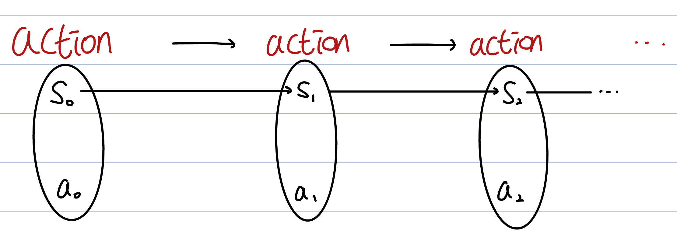
Diagram

Markov Decision Process Diagram³

• \(S_0\): Starting State
  • Subsequent state \(S_1, S_1, \dots, S_n\) changes based on the actions the agent took.
• \(a_0\): Actions taken at \(S_0\)

Properties

1. \(P(a_1 | S_0, a_0, S_1)\): Policy - Distribution of actions at some state. - This policy distribution determines which action to take. - If we know \(S_1\) then we know probability of \(a_1\). No need to know \(S_0\) or \(a_0\) because \(S_1\) contains all the information of \(S_0\) and \(a_0\).

2. \(P(S_2 | S_0, a_0, S_1, a_1)\): Trainsition Probability

   • We need to know \(S_1\) and \(a_1\) as a set to decide the probability of \(S_2\)

Return \(G_t\)

\[G_t \triangleq R_t+\gamma R_{t+1}+\gamma^2 R_{t+2}+\cdots\]

• \(R_t+\gamma R_{t+1}+\gamma^2 R_{t+2}+\cdots\): Sum of discounted rewards
• \(R_{t}\): Reward after doing action \(a_t\)

Learning Objective

Which policy distribution maximizes expected return?

---

1. Figure from this article, Caleb M. Bowyer, Strategies for Decaying Epsilon in Epsilon-Greedy ↩

2. Figure from this article, Renu Khandelwal, Reinforcement Learning: Monte Carlo Method ↩

3. Figure from this article, Tommy Kim ↩