Marcov Decision Process
This post covers Marcov Decision Process in detail, which forms a foundation of Reinforcement Learning. Written in reference to CMU 10401/601 taught by Henry Chai.
Table of contents
- Problem Formulation
- Technical Definition of MDP
- 3 Key Challenges of Reinforcement Learning
- RL Objective Function
- Football Example
Problem Formulation
Terms
- State Space \(S\)
- Action Space \(A\)
- Reward Function
There are two different reward functions that leads to different definitions of the problem at a high-level, but these two functions do the same following thing: Reward function tells you how good some actions is in some state.- Stochastic, \(p(r|s, a)\) Returns distribution over rewards given some state and action.
- Deterministic, \(R: S \times A \rightarrow \mathbb{R}\)
- Transition Function
Every action I take brings me to a new state that can again either be a deterministic function \(f\) or some distribution over next states.- Stochastic, \(p(s’|s,a)\)
- Deterministic, \(\delta: S \times A \rightarrow S\)
- Policy \(\pi: S \rightarrow A\) Specifies an action to take in every state. This that we are trying to learn.
- Value Function \(V^{\pi}: S \rightarrow \mathbb{R}\)
- Some measure of how good the policy \(\pi\) is, given an initial state \(S\)
- Optimal policy maximizes value function in every state.
Technical Definition of MDP
In the context of reinforcement learning, we need to define what’s known as Data Generation Process. The idea is reinforcement learning algorithms, they’re going to require some sort of training data to learn from, but *where does that training data come from?.
- Start in some initial state \(s_0\)
- For time step \(t\):
- Agent observes state \(s_t\)
- Agent takes action \(a_t = \pi(s_t)\) Based on some policy, not necessarily the optimal policy based on some mechanism, it takes an action in that state.
- Agent recieves reward \(r_t \sim p(r | s_t, a_t)\) Recives some reward, here it is written out stochastically, but this could be deterministic.
- Agent transitions to state \(s_{t+1} \sim p(s’ | s_t, a_t)\)
Ends up in some new state.
→ These 2.1 ~ 2.4 creates training data set and are observation in my training data set. Also called as observation tuple.
→ We repeat this until we hit some terminal state or until we reach some time horizon.
- Total reward: \(\sum_{t=0}^{\infty} \gamma{^t} \cdot r_t\)
- In the case of infinite time horizon reward.
- \(\gamma\) = Discount Factor, \(\gamma \in (0,1) \)
3 Key Challenges of Reinforcement Learning
- The algorithm has to gather its own training data.
You need to find some way of gathering this training data such that you are able to learn a reasonable policy from your own training data set. - The outcome of taking some action is often stochastic or unknown until after the fact.
- Room for error that might lead us down sub-optimal paths.
- Decisions can have a delayed effect on future outcomes. (Exploration-Exploitation tradeoff)
- Potential cost in terms of maximizing its current reward.
- The system itself has some incentive to try and chase high reward actions, but that might lead to sub-optimal learning of the system.
- Multi-armed Bandit Problem
Multi-armed Bandit problem(Slot machine problem)
 Multi-armed Bandit Problem Illustration1
- \(|S| = 1\), agent standing infront of slot machines.
- \(A = {1,2,3}\) pull slot machine 1, 2 or 3.
- Deterministic transition
- Rewards are stochastic and unknown to agent
In this context, the agent is going to figure out:
- What those rewards distributions are
- but also what is the sort of the right policy given that distribution over the reward is.
As point 1 and 2 describe, it is not an easy problem to learn optimal solutions while dynamics of the system is unknown.
RL Objective Function
\[\begin{aligned} V^\pi(s) &=E_{p\left(s^{\prime} \mid s, a\right)} {\left[R\left(S_0=s, \pi\left(S_0\right)\right)+\gamma R\left(S_1, \pi\left(S_1\right)\right)\right.} \left.+\gamma^2 R\left(S_2, \pi\left(S_2\right)\right)+\cdots\right] \\ & =\sum_{t=0}^{\infty} \gamma^t E_{p\left(s^{\prime} \mid s, a\right)}\left[R\left(S_t, \pi\left(S_t\right)\right)\right],\ (\text{for some} \ 0<\gamma<1) \end{aligned}\]- Objective: Find a policy \(\pi^*=\underset{\pi}{\arg \max } \ V^\pi(s) \ \forall \ s \in S\)
- \(\pi^*\), optimal policy
- \(V^\pi(s) = E[\text{discounted total reward of starting in state} \ s \ \text{and executing policy} \ \pi \ \text{forever}]\)
- The value of being in some state \(s\) conditioned on, or subject to this policiy \(\pi\) is expected discounted total reward of starting in this state \(s\) and just following the policy \(\pi\) tells you to do in each state.
\(E_{p(s^{\prime})\): This expectation is going to be w.r.t my stochastic transition.
\(\Leftrightarrow\) Distribution over next state \(s’\) given my current state \(s\), and my current action \(a\)
- \(s_0\): Initial state
- \(\pi (s_0)\): Take action \(\pi\) in the state \(s_0\)
- \(\gamma\): Discounted amount
Linearity of expectations Expected value of a sum = equal to the sum of the expected values of each term.
Football Example
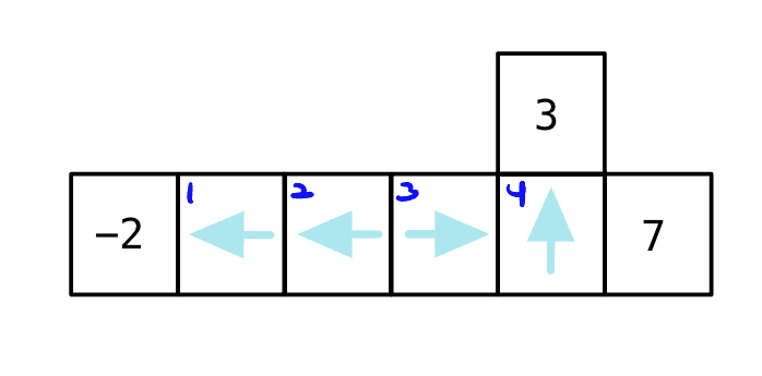
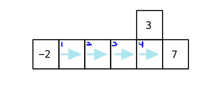
\[R(s, a)=\left\{\begin{array}{c} -2 \ (\text{if entering state 0}) \\ 3 \ (\text{if entering state 5}) \\ 7 \ (\text{if entering state 6}) \\ 0 \ (\text{other wise}) \end{array}\right.\]- Value is always defined relative to some policy.
- Blue arrows in the image represent policies. Under this policy condition, if we calculate reward:
- \(\gamma = 0.9\).
- Using my discount factor, I can actually develop sort of preferences.

State 1: \(-2 + \gamma(0) = -2 \)
State 2: \(0 + \gamma(-2) = -1.8 \)
State 3: \(0 + \gamma(3) = 2.7 \)
State 4: \(3 + \gamma(0) = 3 \)

State 1: \(5.103 \)
State 2: \(5.67 \)
State 3: \(6.3 \)
State 4: \(7 \)
Note that reward values in each of the states across the board are higher under the second policy tha the first one. And this is the equivalence between the optimal policy and the maximul value function. \(\Leftrightarrow\) The optimal policy maximizes the value function in every state.
-
Figure from this webpage, MoanaAkasso ↩